Mathematica简单的三维随机游走及实现
2026-07-19 · Mathematica
阅读栏适合正文;宽栏便于看三维图与长代码。
三维随机游走:每一步在空间中随机选一个方向,位置累加,轨迹在三维里扭来扭去。本文用 Mathematica 把几种直观画法写清楚——立方体堆路径、格点管道、连续方向、动画与统计检验。文中插图均由配套脚本 wolfram/random-walk-3d/random-walk-3d.wls(SeedRandom[20130101])导出,可本地复现。
若关心随机游走在随机过程、强化学习等方向的理论背景,见姊妹篇 随机游走的理论与跨学科应用。
模型约定
离散三维游走可写成
S_0 = 0, S_{k+1} = S_k + X_{k+1}
其中步长 X_i 独立同分布,取值于某个有限方向集(六面邻接、八顶点对角等)。Mathematica 里对应的就是:先定 dirs,再 RandomChoice / Accumulate / FoldList,最后交给 Graphics3D。
方法一:立方体叠加
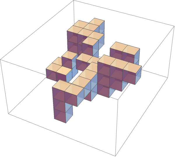
思路:准备单位立方体 Cuboid[],每一步沿六面方向之一平移一格(±e_x, ±e_y, ±e_z),用 FoldList 记下所有变换后的立方体,叠在一起就是游走。
六方向可写成单位矩阵及其相反:
dirs = Join[IdentityMatrix[3], -IdentityMatrix[3]];
(* {1,0,0}, {0,1,0}, {0,0,1}, {-1,0,0}, {0,-1,0}, {0,0,-1} *)
用 FoldList 把平移作用在图形上。GeometricTransformation 配合 TranslationTransform,每步把上一步的立方体再挪一格:
n = 60;
cuboids = FoldList[
  GeometricTransformation[#1, TranslationTransform[#2]] &,
  Cuboid[],
  RandomChoice[dirs, n]
];
Graphics3D[
  {Opacity[0.85], EdgeForm[GrayLevel[0.3]], cuboids},
  Boxed -> True, BoxRatios -> Automatic
]
若更想先拿坐标再画,也可以先累加位移,再批量套变换——语义一样,往往更清晰:
positions = FoldList[Plus, {0, 0, 0}, RandomChoice[dirs, n]];
Graphics3D[
  GeometricTransformation[Cuboid[], TranslationTransform /@ positions]
]
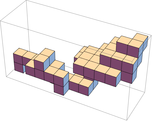
FoldList[Plus, …] 得坐标,再批量 TranslationTransform。体块挨着堆,路径像一条弯折的“积木蛇”,体感很强,适合步数不太多时展示。步数一大,图元过多会变慢,可改用方法二。
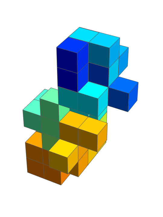
着色:按步序渐变
给每个立方体上色,能看出“时间从哪走到哪”:
positions = FoldList[Plus, {0, 0, 0}, RandomChoice[dirs, 80]];
cols = Blend[{Blue, Cyan, Yellow, Orange}, #] & /@ Rescale[Range[0, Length[positions] - 1]];
Graphics3D[
  MapThread[
    {#1, EdgeForm[GrayLevel[0.35]],
     GeometricTransformation[Cuboid[], TranslationTransform[#2]]} &,
    {cols, positions}
  ],
  Boxed -> False, Lighting -> "Neutral"
]
方法二:格点游走 + Tube
只关心轨迹点,不堆实体。方向取立方体八个顶点方向 Tuples[{-1, 1}, 3],即对角线上的八个格点向量;用 Accumulate 累加随机步长,再用 Tube 画成管道。
dirs = Tuples[{-1, 1}, 3];
(* 八个方向:{±1,±1,±1} 的全部组合 *)

data = Accumulate[RandomChoice[dirs, 200]];
Graphics3D[
  {Orange, Tube[data, 0.35]},
  Boxed -> False, ViewPoint -> {1.3, -2.4, 2}
]
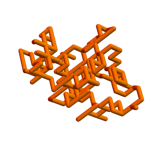
Tube 比折线更有体积感。若希望从原点出发,把原点接到步长序列前面再累加:
data = Accumulate[Prepend[RandomChoice[dirs, 200], {0, 0, 0}]];
Graphics3D[Tube[data, 0.3]]
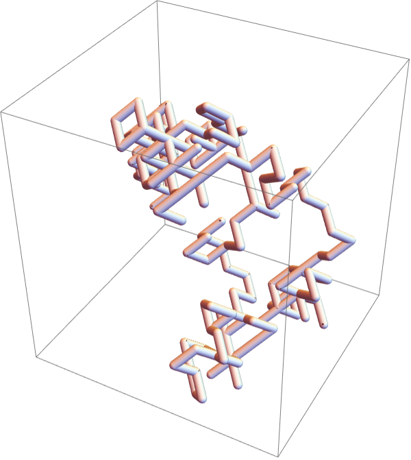
Accumulate。六面邻接格点(与方法一同方向)同样写法,只换 dirs:
dirs = Join[IdentityMatrix[3], -IdentityMatrix[3]];
data = Accumulate[Prepend[RandomChoice[dirs, 300], {0, 0, 0}]];
Graphics3D[{CapForm["Butt"], Tube[data, 0.25]}]
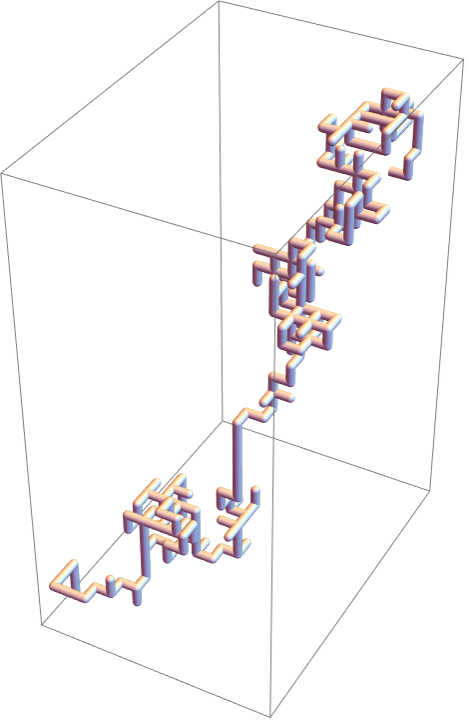
Tube 比 Line 更有体积感;步数上千时仍轻巧,适合长轨迹。
起终点与自交感
dirs = Join[IdentityMatrix[3], -IdentityMatrix[3]];
path = Accumulate[Prepend[RandomChoice[dirs, 400], {0, 0, 0}]];
Graphics3D[{
  {GrayLevel[0.55], Tube[path, 0.2]},
  {Green, Sphere[First[path], 0.55]},
  {Red, Sphere[Last[path], 0.55]}
}, Boxed -> False]
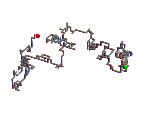
方法三:连续方向(球面随机步)
离散格点之外,可在单位球上均匀取方向,得到更接近布朗运动直觉的折线:
step[] := Normalize @ RandomReal[NormalDistribution[0, 1], 3];
path = Accumulate[Table[step[], 500]];
Graphics3D[
  {ColorData["Rainbow"][0.15], Tube[path, 0.08]},
  Boxed -> False, ViewPoint -> {2, -2, 1.2}
]
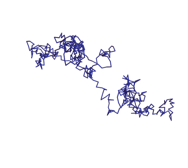
用三维标准正态再归一化,方向在球面上近似均匀(高斯向量的旋转对称性)。若要固定步长 δ,写成 δ * step[] 即可。
方法四:有偏游走与受限区域
现实模型里步长往往不对称,或被边界挡住。下面给一个向 +z 略偏、并限制在盒子内的版本:
dirs = Join[IdentityMatrix[3], -IdentityMatrix[3]];
weights = {1, 1, 1.4, 1, 1, 0.7}; (* +z 更易被选中 *)
box = Cuboid[{-8, -8, -8}, {8, 8, 8}];

insideQ[p_] := And @@ Thread[-8 <= p <= 8];

biasedStep[p_] := Module[{cand},
  cand = p + RandomChoice[weights -> dirs];
  If[insideQ[cand], cand, p]
];

path = NestList[biasedStep, {0, 0, 0}, 600];
Graphics3D[{
  {Opacity[0.08], EdgeForm[None], box},
  {Orange, Tube[path, 0.22]},
  {Red, Sphere[Last[path], 0.4]}
}, Boxed -> False]
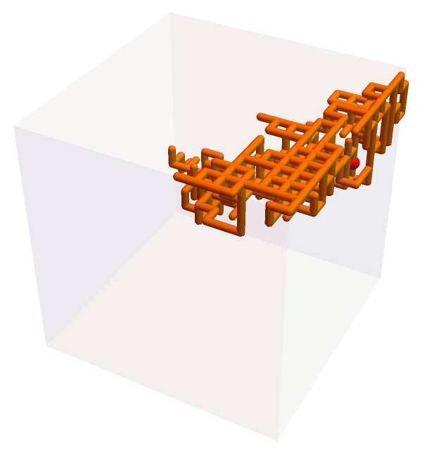
+z 略偏、撞墙停留;轨迹整体上浮并被盒子约束。撞墙时停在原地(反射/吸收可再改);权重一调,轨迹就会整体“往上漂”。
动画:一步步长出来
dirs = Join[IdentityMatrix[3], -IdentityMatrix[3]];
path = Accumulate[Prepend[RandomChoice[dirs, 120], {0, 0, 0}]];

Animate[
  Graphics3D[
    {CapForm["Round"], Tube[Take[path, k], 0.28],
     Red, Sphere[path[[k]], 0.45]},
    PlotRange -> (MinMax /@ Transpose[path]),
    Boxed -> False, SphericalRegion -> True
  ],
  {k, 2, Length[path], 1},
  AnimationRate -> 12
]
笔记本里用 Animate;脚本侧用帧序列导出 GIF(无前端亦可复现):

统计:均方位移
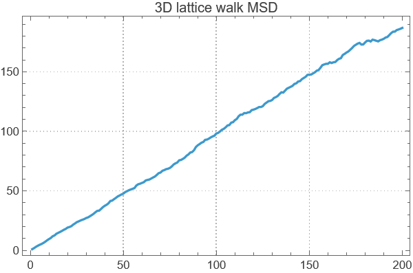
对称格点游走在大步数下,均方位移应近似线性增长:⟨|S_n|²⟩ ∝ n。用多条轨迹验证:
dirs = Join[IdentityMatrix[3], -IdentityMatrix[3]];
n = 200; trials = 400;

msd = Mean @ Table[
  With[{path = Accumulate[RandomChoice[dirs, n]]},
    Total /@ (path^2)  (* |S_k|² 随 k *)
  ],
  {trials}
];

ListLinePlot[msd,
  AxesLabel -> {"n", "⟨r²⟩"},
  PlotLabel -> "3D 格点游走:均方位移",
  PlotTheme -> "Detailed"
]
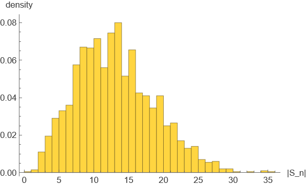
单条轨迹的末端距离分布也可看一眼:
ends = Table[
  Norm @ Total @ RandomChoice[dirs, 200],
  {2000}
];
Histogram[ends, 40, "PDF", AxesLabel -> {"|S_n|", "密度"}]
一点对比
| 立方体叠加 | 格点 + Tube | 球面连续步 | |
|---|---|---|---|
| 数据 | 变换后的 Cuboid | 坐标列表 | 坐标列表 |
| 方向 | 常取六面 | 六面或八顶点 | 单位球连续 |
| 观感 | 积木感、占空间 | 细管轨迹、步数可更大 | 更“布朗” |
| 核心函数 | FoldList + TranslationTransform | Accumulate + Tube | Normalize + Accumulate |
| 适用 | 短路径演示 | 长轨迹 / 动画 | 连续模型直觉 |
小封装
日常试错时可以收成一个函数:
RandomWalk3D[n_, opts : OptionsPattern[Graphics3D]] := Module[
  {dirs = Join[IdentityMatrix[3], -IdentityMatrix[3]], path},
  path = Accumulate[Prepend[RandomChoice[dirs, n], {0., 0., 0.}]];
  Graphics3D[
    {ColorData["SolarColors"][0.55], CapForm["Round"], Tube[path, 0.25]},
    Boxed -> False, SphericalRegion -> True, opts
  ]
];

RandomWalk3D[300, ViewPoint -> {1.4, -2.2, 1.5}]
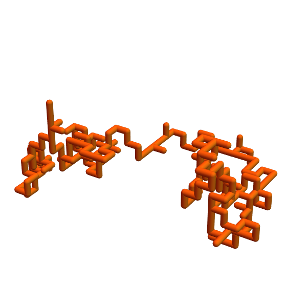
RandomWalk3D[300] 一键出图。方向集、权重、边界、着色都可以做成选项,按需要再拆。完整脚本与输出目录见 wolfram/random-walk-3d。
小结
两种经典写法——FoldList 堆立方体、与 Accumulate + Tube——已经够把三维随机游走在笔记本里画出来。再加上连续步、有偏/受限、动画和均方位移,就能从“好看”走到“能检验模型”。改方向集、步数和样式做实验时,优先用坐标列表那条路,扩展成本最低。
这篇文章的渊源
方法一并非凭空发明。Wolfram Language 文档 TranslationTransform 里就有一条示例,标题正是 “A random translation walk”:用 FoldList 把 GeometricTransformation[..., TranslationTransform[#2]] 反复作用在 Cuboid[] 上,方向由 RandomChoice 给出。本文 2013 年记下的,就是把这条文档套路拆开讲清楚——六面方向怎么写、先累加坐标再批量变换为何更清晰——再补上 Tube / Accumulate 的格点画法,以及后来加上的连续步、有偏与统计检验。可以说:文档给了“一行能跑的种子”,这篇是把它展开成可改、可验的笔记。
Fold 与 FoldList 展开
游走的数学是 Sk+1 = f(Sk, Xk+1)。Mathematica 里:
Fold[f, x, {a, b, c}]
(* → f[f[f[x, a], b], c]  只要终值 *)

FoldList[f, x, {a, b, c}]
(* → {x, f[x,a], f[f[x,a],b], f[f[f[x,a],b],c]}  全程快照 *)
方法一要的是整条轨迹上的图形,所以用 FoldList;若只要终点立方体,改 Fold 即可。FoldList[Plus, {0,0,0}, steps] 与 Accumulate[Prepend[steps, {0,0,0}]] 在加法情形下等价——Accumulate 是“二元运算固定为 Plus”的特化;一旦 f 变成几何变换合成,就必须回到一般的 Fold / FoldList。
(* 与本文方法一同一骨架 *)
FoldList[
  GeometricTransformation[#1, TranslationTransform[#2]] &,
  Cuboid[],
  RandomChoice[dirs, n]
]
计算机科学与函数式内涵
在函数式编程里,这叫 fold(亦称 reduce、inject):用一个二元运算把列表“折”进累加器。它是列表上的catamorphism——结构性递归的标准形态:对空列表给初值,对 x :: xs 做 f(x, fold(xs))(右折)或对称的左折。随机游走、前缀和、状态机步进、解析器组合子,本质都是“状态 × 输入 → 新状态”的左折;FoldList 则多露出中间状态,对应 scan / prefix 一族,正好服务可视化与调试。
相对命令式 for 循环就地改坐标,fold 把更新规则收成参数 f:换方向集、换有偏权重、换边界策略,往往只改 f 或列表,不改控制流。这也是本文方法一能从“平移立方体”平滑扩到“任意几何变换序列”的原因。
其它语言里的近亲
| 语言 / 库 | 只要终值(≈ Fold) | 要中间结果(≈ FoldList) |
|---|---|---|
| Haskell | foldl / foldr | scanl / scanr |
| OCaml / F# | List.fold_left | 自写 scan,或 Seq.scan(F#) |
| Scala | foldLeft | scanLeft |
| Python | functools.reduce | 手写循环,或 itertools.accumulate(限加法等) |
| JavaScript | array.reduce | 自写;无内置 scan |
| Rust | Iterator::fold | scan(闭包里可变状态) |
| C++ (STL) | std::accumulate | std::partial_sum(偏数值) |
| NumPy | — | numpy.cumsum(加法特化,≈ Accumulate) |
格点游走在别处常写成 cumsum(random_steps);立方体叠加那种“f 是几何变换”的版本,在多数语言里没有现成的 GeometricTransformation,但 fold/scan 骨架一样——累加器换成变换矩阵或位姿即可。读文档示例、用 FoldList 画积木蛇、再对照上表换语言重写一遍,是把这篇笔记从 Mathematica 语法迁到通用计算思维的最短路径。